Missing Data
Missing data is a common occurrence in research and is unfortunately often ignored. Most software drops the missing data to be helpful. However, by dropping that data we assume that data is missing completely at random. This is often an unreasonable assumption and often unlikely to be true. While missing data may have a negligible effect when only a few observations are missing, this is not always the case if there is substantial missing data.
We will describe inverse probability weighting approaches to account for missing data. We will detail inverse probability of missing weights for different patterns of missing data, and inverse probability of censoring weights (a special case of IPMW). Note: I am neglecting to mention multiple imputation, which is another approach to handling data.
IPMW
Inverse probability of missing weights are one way to account for missing data. IPMW works by reweighting the observed sample to reflect the full data. IPMW can be calculated for any missing variable in the data. To help frame the discussion of missing data, consider the following data sets
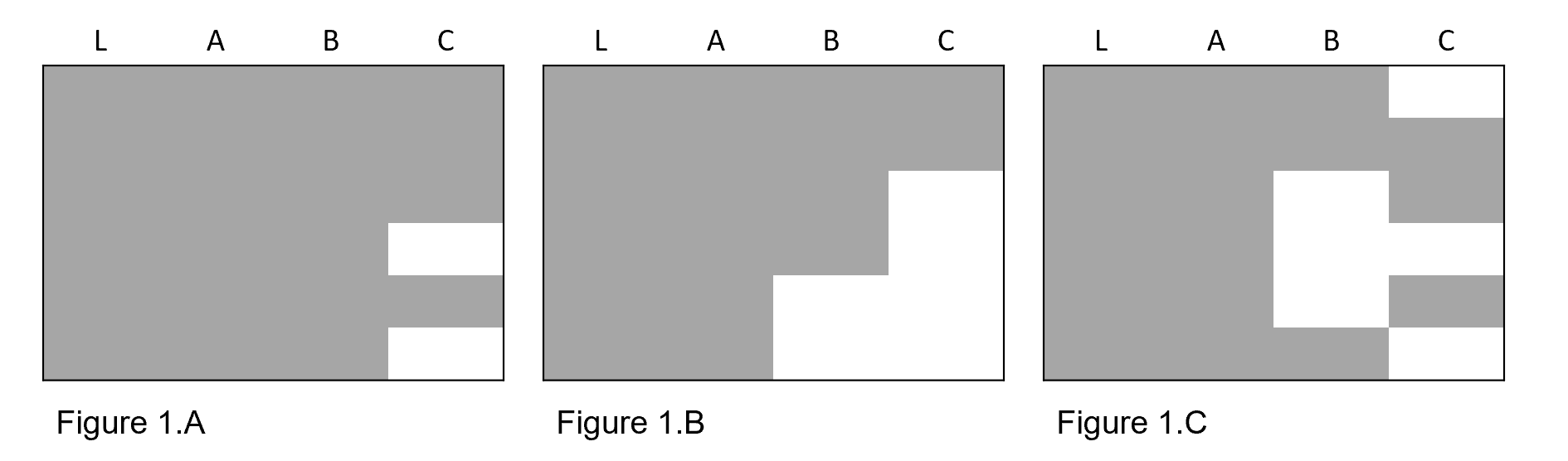
Figure 1.A summarizes missing data for a single variable. Single variables only require a single IPMW estimation step. Figure 1.B is an example of monotonic missing data. For monotonic missing data, if one variable is missing (B), then the the next missing variable must also be missing (C). In this scenario, we use an iterative process of calculating IPMW. Lastly, there is non-monotonic missing data. Non-monotonic missing data does not follow the pattern of monotonic missing data. A variable missing for one column may or may not be missing for another. This is more complex to solve and likely more common in practice.
Single Variable
First, we will focus on the case shown in Figure 1.C, missing data for a single variable. We will load the sample simulation data. Loading the simulated data
from zepid import load_sample_data
from zepid.causal.ipw import IPMW
df = load_sample_data(timevary=False)
The missing variable is this data set we will focus on is dead. Since dead is our outcome in later analyses, these weights could also be referred to as inverse probability of censoring weights. However, we will use IPMW to calculate weights for outcomes measured at a single time.
In this example, we will assume data is missing completely at random conditional on age, ART, and gender. Additionally, we will stabilize the weights and include ART in both the denominator and numerator. This weight formation is useful for later analyses our the average causal effect of ART on death. Please see the tutorials on Time-Fixed Exposures for further information (I leave it to the reader to merge IPMW with the methods described in Time-Fixed Exposures)
ipm = IPMW(df, missing='dead', stabilized=True)
ipm.regression_models(model_denominator='age0 + art + male',
                      model_numerator='art')
ipm.fit()
After calculating our weights, we can save the calculated weights for later usage
df['ipmw'] = ipm.Weight
Additionally, we don’t necessarily need to use monotonic IPMW if we have data as shown in Figure 1.B. We may be willing to assume that C’s missingness does not depend on B. In that scenario, we could calculate two sets of IPMW following the above procedure. Then we would multiply the two sets of weights to obtain our final set of IPMW. If we are not willing to assume that C missing does not depend on B, we will need to use the IPMW formulation described in the following section. That concludes IPMW for a single missing variable.
Monotone Missingness
For this next tutorial, we will load another simulated data. In this data set, there are four variables. Two of the variables are missing (B and C) and follow the pattern shown in Figure 1.B
from zepid import load_monotone_missing_data
from zepid.causal.ipw import IPMW
df = load_monotone_missing_data()
For monotonic missing data, we use a similar process. However, we provide a list of missing variables instead of a single string. Additionally, we specify a list of regression models. Specifically, we assume that B is missing completely at random given L and A. We assume C is missing completely at random given L and B. Since C depends on B and B is missing, we need to use this iterative process to calculate IPMW.
ipm = IPMW(df, missing_variable=['B', 'C'], monotone=True)
ipm.regression_models(model_denominator=['L + A', 'L + B'])
ipm.fit()
Behind the scenes, the model for B is fit, C is fit, then the calculated weights are multiplied together to obtain our full IPMW set. Again, we can set the calculated weights as a variable in our data for later use
df['ipmmw'] = ipm.Weight
There is also a special case of monotonic data missing data. If variable C was always missing when B was missing in Figure 1, then the monotonic IPMW becomes the same as single-variable IPMW. Behind the scenes, IPMW checks for this special case and uses the single-variable process if it detects it. You can manually do this by only specifying one of the missing variables
Non-Monotone Missingness
Non-monotonic missing data is not currently supported. Future plans are to include IPMW for non-monotonic data
AIPMW
Augmented-IPMW is a doubly robust procedure to account for missing data. This is not currently implemented but is planned for the future. This expands to the same scenarios that IPMW does
IPCW
As mentioned in the introduction, inverse probability of censoring weights can be viewed as a special case of missing data. Specifically, censoring is missing data on the outcome. Additionally, censored data will generally follow a monotone missing pattern (once a participant is censored, they are censored for all future time points).
IPCW is built to accounting for censoring in time-to-event data. For missing outcome data at a single follow-up time, IPMW should be used instead. For the IPCW tutorial, we will use the time-varying simulated sample data. To motivate this example, we are interested in estimating the overall risk of mortality over time. However, we are concerned about censoring being dependent on gender and age.
We will load the data via
from zepid import load_sample_data, spline
from zepid.causal.ipw import IPCW

df = load_sample_data(True)
df[['age_rs1', 'age_rs2']] = spline(df, 'age0', n_knots=3, term=2, restricted=True)
df[['enter_rs1', 'enter_rs2']] = spline(df, 'enter', n_knots=3, term=2, restricted=True)
After loading our data, we can calculate IPCW with the following code. For IPCW, it is recommended to use stabilized weights. We will stabilize our weights by time (enter), which is common practice
ipcw = IPCW(df, idvar='id', time='enter', event='dead')
ipcw.regression_models('enter + enter_rs1 + enter_rs2 + male + age0 + age_rs1 + age_rs2',
                      model_numerator='enter + enter_rs1 + enter_rs2',
                      print_results=False)
ipcw.fit()
Finally, we can add these weights to our data set.
df['cw'] = ipcw.Weight
Now, we can estimate a weighted Kaplan-Meier to obtain the risk curve, allowing for non-informative censoring conditional on age and gender
Summary
This concludes the discussion of approaches to account for missing data with zEpid. Please see the online tutorials at this GitHub repo for further descriptions and examples